Spectral Pre-processing: Difference between revisions
m (→Cut) |
|||
| (One intermediate revision by the same user not shown) | |||
| Line 18: | Line 18: | ||
== Baseline subtraction == | == Baseline subtraction == | ||
:[[File:baselinecorr.jpg|right|frame|Screenshot of the dialog box ''baseline correction'']] | |||
The function divides a spectrum into segments, or intervals, for each of which a minimum MS intensity value is determined. These values are then used to generate a baseline correction curve (by shape preserving piecewise cubic interpolation). The interpolated baseline correction curves are subtracted from the original spectra. | The function divides a spectrum into segments, or intervals, for each of which a minimum MS intensity value is determined. These values are then used to generate a baseline correction curve (by shape preserving piecewise cubic interpolation). The interpolated baseline correction curves are subtracted from the original spectra. | ||
| Line 48: | Line 50: | ||
Normalization does not require parameters. The normalization function is available from the ''Preprocessing'' pulldown menu or via the button normalize in the ''PREPROCESS'' tab. | Normalization does not require parameters. The normalization function is available from the ''Preprocessing'' pulldown menu or via the button normalize in the ''PREPROCESS'' tab. | ||
== Reduce resolution == | == Reduce resolution (binning) == | ||
:[[File:redes.jpg||right|frame|Screenshot of the window ''reduce resolution'']] | :[[File:redes.jpg||right|frame|Screenshot of the window ''reduce resolution'']] | ||
Latest revision as of 21:04, 6 April 2025
Introduction
Spectral data analysis is a challenging task in the MALDI-ToF MS-based workflow for microbial identification. Considering that a MALDI-ToF mass spectrum is a complex signal, typically containing between 80 to 150 peaks and noise contributions, adequate spectral pre-processing is highly beneficial prior to peak detection and identification, or classification analysis.
The quality of microbial mass spectra should be assessed visually immediately after data acquisition using the following criteria: first and foremost, the signal-to-noise ratio (SNR) and the presence of a sufficient number of mass peaks. Other quality criteria include a relatively flat shape of the spectral baseline and the absence of interfering or confusing mass peaks from plasticisers or other synthetic polymer additives. Outliers, i.e. spectra that do not meet one or more of the quality criteria, should not be accepted for multivariate classification analysis and should be excluded from further analysis.
Aside from assessing the spectral quality visually, quality testing can be carried also by means of the function MALDI quality test (QT).
Autocalibration
 Screenshot of the dialog box autocalibration

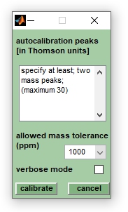
Performs linear recalibration of mass spectra using internal calibration peaks for which precise m/z positions are required. Note that non-linear methods are not available. Auto-calibration overwrites existing pre-processed spectra and modifies also existing peak tables. If no pre-processed spectra are available auto-calibration will create pre-processed spectra from the original mass spectra, i.e. the original spectra are not modified by this function.
The spectral pre-processing procedure of auto-calibration is based on the use of analyte mass peaks, i.e. it requires the knowledge of the precise peak positions of at least two different sample peaks per mass spectrum. To perform auto-calibration, it is necessary to generate peak tables from appropriately pre-processed mass spectra. After peak detection, select the spectra to be calibrated and choose autocalibrate from the Preprocessing pulldown menu.
This will open a dialog box entitled autocalibration of mass spectra. Enter the exact m/z positions of at least 2 and no more than 30 mass peaks and set the estimated calibration error from the allowed mass tolerence (ppm) popupmenu. Select larger values (>1000 ppm) if you are unsure of the actual calibration error. The pseudo-gel view can be helpful in defining the positions of peaks suitable for auto-calibration. Press calibrate when finished.
IMPORTANT: At least two of the peaks used for autocalibration should have counterparts in the peak tables of the uncalibrated spectra. It is worth checking the output of the command line window when autocalibration has finished.
The parameters used for autocalibration are stored within the program workspace and are accessible from the FILE INFO tab (press button edit of the FILE INFO tab, or select edit header info from the Edit pulldown menu).
Baseline subtraction
 Screenshot of the dialog box baseline correction

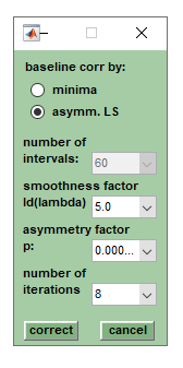
The function divides a spectrum into segments, or intervals, for each of which a minimum MS intensity value is determined. These values are then used to generate a baseline correction curve (by shape preserving piecewise cubic interpolation). The interpolated baseline correction curves are subtracted from the original spectra. To perform baseline correction, first select the spectra to be corrected from the listbox in the top right corner (Screenshot of MicrobeMS). Then select the number of intervals from the popup menu # of intervals in the VIEW tab. Valid values for the number of intervals (niv) are 3, 5, 7, 9, 11, 13, 15, 17, 19, 21, 23, 25, 27, 29, 31, 35, 45, 55, 65 and 75. Subsequently press the baseline button (VIEW tab). If the checkbox org. spectra is selected baseline correction will create pre-processed spectra from original spectra. Note that existing pre-processed spectra will be overwritten without warning in this case. To perform baseline correction from existing pre-processed spectra, clear the org. spectra checkbox .
Baseline correction should be repeated from the original spectra if negative intensities occur after baseline correction. For this purpose the checkbox org. spectra should be ticked and the parameter # of intervals should be reduced to 60 or less. Again, existing pre-processed spectra will be overwritten without warning.
The parameters used for baseline correction are stored within the program workspace and are accessible from the FILE INFO tab (press button edit on the FILE INFO tab, or select edit header info from the Edit pulldown menu).
With MicrobeMS version 0.87 the function baseline correction by asymmetric least squares (AsLS) has been added as the default baseline correction method. A description of the AsLS algorithm and the meanings of the parameters can be found in the following publication:
 P.H. Eilers and H. F. M. Boelens. Baseline Correction with Asymmetric Least Squares Smoothing.
 Leiden University Centre Medical Report 1(1) 2005 p. 5.
Smoothing
This function is used to smooth mass spectra using the Savitzky-Golay smoothing filter. Smoothing has a largely cosmetic effect on the spectra, reducing the noise at the expense of lowering the resolution of mass peaks. Possible values for smoothing points range between 3 and 75, cf. popupmenu # smooth pts in the PREPROCESS tab of the main window of MicrobeMS. If the checkbox org. spectra is checked smoothing will create pre-processed spectra from original spectra. Note that existing pre-processed spectra will be overwritten without warning in this case. Press the smooth button to smooth selected mass spectra.
Details of the Savitzky-Golay algorithm can be found in the literature:
 A. Savitzky and M. Golay. Smoothing and Differentiation of Data by Simplified Least Squares Procedures.
 Anal. Chem. 1964 Vol 36(8):1627.
The parameters used for smoothing are stored within the program workspace and are accessible from the FILE INFO tab (press button edit of the FILE INFO tab, or select edit header info from the Edit pulldown menu).
Normalization
This function normalizes mass spectra by means of a modified 1-norm algorithm. Normalization is carried out in the following way: The mass spectrum is first subdivided into bins, usually 100, in the m/z range between mzstart and mzstart + 3/5*(mzend- mzstart). For example, if a spectrum spans the m/z range 2000 to 20000, the range between m/z 2000 and 12800 is subdivided into 100 bins. The minimum and maximum intensity values are then obtained from each bin. The next steps are to calculate the intensity difference values for each individual m/z bin and to extract the 16 highest intensity difference values. From these values the 3 largest values are deleted before the sum of the remaining 13 intensity difference values is calculated. Finally, this sum is divided by 1000 and the ratio is used as the normalization factor.
Spectral normalization is achieved by dividing the spectral intensities by the normalization factor.
Normalization does not require parameters. The normalization function is available from the Preprocessing pulldown menu or via the button normalize in the PREPROCESS tab.
Reduce resolution (binning)
 Screenshot of the window reduce resolution

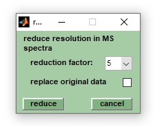
This function allows the effective spectral resolution of mass spectra to be reduced by an arbitrary factor. For large data sets this can be useful to free up some memory before performing memory consuming calculations. Select the data reduction factor from the reduction factor popupmenu, allowed values range from 3 to 21, and press reduce to start the procedure. Press cancel to exit the function. If the checkbox org. spectra is checked (see VIEW tab/main window), reduce resolution will overwrite existing pre-processed spectra without warning. If no pre-processed spectra are available, reduce resolution created pre-processed spectra from original mass spectra. Select the checkbox replace original data to also allow modifications of original spectra. Note that modified original spectra cannot be reverted to their original state (see also the clear pre-processing function).
Cut

Cutting (truncating) mass spectra is useful to narrow the m/z range covered by the mass spectra. For large data sets this can be useful to free up some memory before performing memory consuming calculations. Define the mass range to be retained [m/z], then press the cut button to start the function. Quit the function by pressing the cancel button. If the check box org. spectra is checked (see the VIEW tab in the main MicrobeMS user interface), cut will overwrite existing pre-processed spectra without warning. If no pre-processed spectra exist, cut will create pre-processed spectra from original mass spectra. Check the checkbox cut original data to allow cutting also the original spectra. Note that cutted original spectra cannot be restored to their original state (see also the clear preprocessing function).
The parameters used by the cut function are stored in the program workspace and are accessible via the FILE INFO tab (press the edit button of the FILE INFO tab or select edit header info from the Edit pulldown menu).
Undo pre-processing
This option can be used to delete selected pre-processed mass spectra from the MicrobeMS workspace. Note that original spectra processed by the functions cut and reduce resolution cannot be returned to their original state. The function undo pre-processing is available from the Pre-processing pulldown menu.