Microbial Identification based on Mass Spectral Libraries and Interspectral Distances

Mar 2025: This section describes the microbial identification routine of an outdated version of MicrobeMS (v.085). An updated description of the routine for the latest version of MicrobeMS (v.089) is currently being prepared.

Introduction

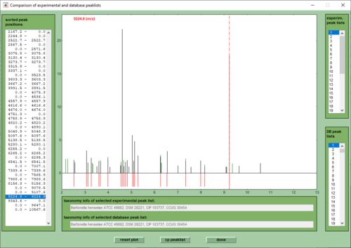
• In the MicrobeMS software package microbial identification based on mass spectral libraries and interspectral distances, or similarity measures such as D-values, is carried out by means of the subfunction cmpr (compare). The cmpr function is available from the Analysis menu bar (select compare with database), or by pressing the button compare with DB in the ANALYSIS tab (see Screenshot of MicrobeMS). The function calculates interspectral distances (on the basis of peak tables) between spectra in a database and the experimental mass spectra. Spectra in a database, also called reference spectra, are recorded from microorganisms with a known taxonomic status and can be of two types: (i) single experimental spectra and (ii) so-called database spectra. The latter are created from a selection of experimental spectra (see section interspectral distances below).

Screenshot of the dialog box "Identification analysis based on interspectral distances"

Screenshot of the window "Show db content (in silico database)"

Screenshot of the dialog box "More results (Debian Linux)"

• Reference spectra are ranked by the cmpr function according to their spectral distances to the test spectrum such that the reference spectrum with the smallest distance (or highest score) appears on the top of the ranking list. As the genus, species and strain identity of the microorganisms used to record the database spectra are known, this allows microbial identification at certain taxonomic level.

• In MicrobeMS spectral distances can be obtained by using different metrices: Euclidean distances, D-values derived from Pearson’s product-momentum correlation coefficients, covariance and Pareto scaling (see section interspectral distances below). All distance algorithms search for matching peaks in the peak tables of the test spectra and the spectra comprising the database, respectively.

• The function cmpr always requires the presence of peak tables. These peak tables must be obtained from both types of spectra, test and reference spectra. Peak tables contain the m/z positions of the peaks, intensities of the unprocessed spectra, normalized intensities (also called weightings) and – in case of database spectra – frequency values of the mass peaks. Frequency values indicate how often a peak was found in the experimental spectra used to create the actual database spectrum.

• An important problem of calculating interspectral distances from different MALDI TOF mass spectra is to define the conditions at which a peak in the test spectrum matches a peak in a reference spectrum. It is known that MALDI TOF MS generally suffers from a relatively low precision of the experimentally determined m/z peak positions. Therefore, when analyzing spectra from biological and technical replicates mass peaks of theoretically identical m/z positions may be detected at slightly varying m/z positions. To deal with such inaccuracies of the m/z positions, a program wide variable ppm has been introduced. The ppm parameter defines the maximum allowed variation between theoretically identical peaks obtained by different measurements. The ppm variable defines the width of mass regions, or m/z sections (intervals), in which spectra are subdivided: [M-ppm/2 M+ppm/2], with M being the m/z position of a given section center. Only in cases where peaks from distinct spectral measurements fall within the borders of such m/z sections they are treated as identical peaks.

• Database spectra are ideally created from a defined number of experimental mass spectra, usually between 3 and 20. The procedure of creating database spectra always starts from raw experimental mass spectra and includes spectral pre-processing, peak detection followed by a statistical analysis of the peak tables. A database spectrum is essentially represented by a peak table in which the following values are stored:

a) the average peak position of mass peaks,
b) the mean intensities of the mass peaks (obtained from experimental mass spectra),
c) normalized peak intensities (weightings): the sum of the normalized intensities equals 100 in a database spectrum and
d) the frequency the peaks are found in the experimental mass spectra used to create the database spectrum.
    (see also format of peak tables)

• Parameters for automated spectral pre-processing and peak detection are stored in the file microbems.opt. This file is a simple text file which can be edited by text editors like Notepad. It is required to restart MicrobeMS to initialize changes made to this file. Note that existing blocks of pre-processed spectra, or peak tables are not overwritten when creating database spectra from experimental mass spectra.

Interspectral distances

In MicrobeMS, interspectral distances are calculated from peak tables (see above) and can be of the following types:

1. Euclidean distances: probably the most commonly chosen type of distance. The Euclidean distance can be considered the geometric distance in a multidimensional space, see Euclidean distance for details.
 

2. Pearson: Pearson distances $D_{1}(x,y)$ between two peak tables x and y are calculated on the basis of Pearson's product momentum correlation coefficient, which is basically the covariance $cov(x,y)$ divided by the product of their standard deviations $\sigma _{x}\sigma _{y}$, this product is also known as the total joint variance. Values of $r_{1}(x,y)$ may vary between -1 (perfect negative linear correlation), 0 (no correlation) and 1 (perfect positive linear correlation). Equation (2) is then applied to obtain Pearson's distance $D_{1}(x,y)$. This distance varies between 0 (identity - perfect positive linear correlation) and 2000 (anti-correlation - perfect negative linear correlation).
    
   

   $r_{1}(x,y)={cov(x,y) \over \sigma _{x}\sigma _{y}}$ (1), and $D_{1}(x,y)=1000*[1-r_{1}(x,y)]$ (2)

 

3. Pareto (0.75): The Pareto-0.75 distance $D_{0.75}(x,y)$ between two peak tables x and y is obtained on the basis of the Pareto-scaled correlation coefficient $r_{0.75}(x,y)$ which is calculated by dividing the covariance cov(x,y) of the two vectors by the product of their standard deviations to the power of 0.75, see eqn. (3). Resulting values are then scaled by dividing them by $r_{0.75}(x,x)$. For this purpose, the test peak table vector is compared with itself. $D_{0.75}(x,y)$ can be subsequently computed from equation (4). Note that the Pareto-0.75 distance can be smaller than 0 and larger than 2000.
    
   

   $r_{0.75}(x,y)={cov(x,y) \over (\sigma _{x}\sigma _{y})^{0.75}}$ (3), and $D_{0.75}(x,y)=1000*[1-{r_{0.75}(x,y) \over r_{0.75}(x,x)}]$ (4)

 

4. Pareto (0.50): The Pareto-0.50 distance $D_{0.50}(x,y)$ between two peak tables x and y is determined in a similar way to the Pareto-0.75 distance: The only difference is that the exponent value of 0.75 is replaced by a value of 0.50, cf. eqn. (5) below. Specifically, the Pareto-0.50 distance $D_{0.50}(x,y)$ is obtained on the basis of the Pareto-scaled correlation coefficient $r_{0.50}(x,y)$ which is calculated by dividing the covariance cov(x,y) of the two vectors by the product of their standard deviations to the power of 0.50. $r_{0.50}(x,y)$ values are then scaled by dividing them by $r_{0.50}(x,x)$. For this purpose, the test peak table vector is compared with itself. $D_{0.50}(x,y)$ can be subsequently computed from the following equation (6). Again, the Pareto distance can be smaller than 0 and larger than 2000.
    
   

   $r_{0.50}(x,y)={cov(x,y) \over (\sigma _{x}\sigma _{y})^{0.50}}$ (5), and $D_{0.50}(x,y)=1000*[1-{r_{0.50}(x,y) \over r_{0.50}(x,x)}]$ (6)

 

5. Pareto (0.25): The Pareto-0.25 distance $D_{0.25}(x,y)$ between two peak tables x and y is determined similarly to the Pareto-0.75 distance: The only difference is that the exponent value of 0.75 is replaced by a value of 0.25 (see above). Like the Pareto-0.75 and the Pareto-0.50 distances, values for $D_{0.25}(x,y)$ can be smaller than 0 and larger than 2000.
    
   

   $r_{0.25}(x,y)={cov(x,y) \over (\sigma _{x}\sigma _{y})^{0.25}}$ (7), and $D_{0.25}(x,y)=1000*[1-{r_{0.25}(x,y) \over r_{0.25}(x,x)}]$ (8)

 

6. Covariance: First, the covariance cov(x,y) between the two peak table vectors x and y is calculated. Then, the covariance cov(x,x) between the test peak table vector with itself is obtained. The covariance-based distance $D_{0}(x,y)$ is determined by equation (9). Covariance-based distances can be smaller than 0 and larger than 2000.
    
   

   $D_{0}(x,y)=1000*[1-{cov(x,y) \over cov(x,x)}]$ (9)

 

Scores

Score values $S_{i}$ and log score values $Sld_{i}$ are directly computed from the inter-spectral distance values ($D_{1},D_{0.75},D_{0.50},D_{0.25}$ and $D_{0}$) by means of the following equations:
 

$S_{i}=1000-D_{i}$, if $S_{i}<1$ → $S_{i}=1$ (10), and $Sld_{i}=log_{10}(S_{i})=log_{10}(1000-D_{i})=3-log_{10}(D_{i})$, if $Sld_{i}<0$ → $Sld_{i}=0$ (11)
 

In consequence values of $S_{i}$ vary between 1 (negative, no, or almost no correlation) and 1000 (perfect correlation). $S_{i}$ can be larger than 1000 in cases of Pareto or covariance scaling and if w-fact has been set to values larger than 0 (requires an activated checkbox use weightings).
Computation of logarithmic score values $log_{10}(D_{i})$ produces values between 0 (negative, no, or almost no correlation), 3 (identity), or above 3 (possible only in case of Pareto and covariance scaling). In MicrobeMS score and log score values are helpful to assess and compare levels of similarity between the experimental test spectra and microbial reference spectra, i.e. database spectra.

Score values obtained by MicrobeMS should not be compared to the score values of Bruker's MALDI Biotyper. Due to the different algorithms used - MicrobeMS score values are based on interspectral distances - MicrobeMS scores tend to be larger than the corresponding MALDI Biotyper score values. Of note, such higher scores do not indicate better matches between the experimental test and the database spectra.

It is also important to be aware of the fact that the score values are dependent on the number of peaks in both the test and the database spectra. If the number of peaks is different, the equations used will tend to calculate lower score values. If the underlying MALDI-ToF mass peak tables are of different lengths, this will inevitably lead to reduced correlation values and therefore lower scores. Therefore, it is important that only peak tables are used for the calculation of the score values, in which the number of peaks in all test and database spectra is identical. Otherwise, the identification of microorganisms on the basis of score-ranking lists can lead to erroneous results.

Peak number corr factor (still experimental!): A factor for a still highly experimental procedure to compensate for different numbers of peaks derived from experimental test and database spectra. Obviously, the ratio between the peak numbers of the test and database spectra has a strong influence on the distance values and thus on the calculated scores. It is recommended to select a factor of 1 (default) to disable this algorithm.

Screenshot of the window "MicrobeMS identification report" in the text format

Screenshot of the window "MicrobeMS identification report" (HTML formatted)

Vary calibration parameters

The program option vary calibration parameters allows the three calibration constants c0, c1, and c2 of test time-of-flight mass spectra to be varied in combination. This option generates a larger number n of mass spectra from a single test spectrum, which are then compared against the database spectra. From the n scores obtained, either a top score or the average of a few top scores is selected for the score ranking list. The procedure aims to largely eliminate errors that may arise due to insufficient calibration of the test spectra. The method is quite computationally intensive, but longer program runtimes could be significantly reduced by a suitable programming technique (vectorization of the underlying Matlab code).

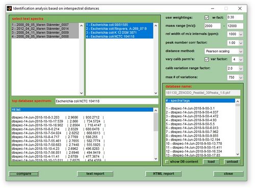
Vary calibration parameters (checkbox): Calibration parameters are varied when this checkbox is activated. When calculating distance values between test and reference spectra, the comparison is done for a set of [2n+1 × 2n+1] variations of three calibration constants, with n being the value chosen from the pull down menu var factor (see screenshot at the top of this page). For example, if the default value of n=4 has been selected from the pull down menu, MicrobeMS will calculate in each comparison interspectral distances between the respective reference spectrum and 729 test spectra [9 × 9 × 9 = (2×4+1) × (2×4+1) × (2×4+1)] representing the different combinations of three different calibration constants c0, c1, and c2. In the easiest case (when the checkbox average distances is unchecked), identification reports will display only one - the best (highest) - match for each test spectrum.
Vary calibration range factor: This factor defines the range in which the calibration constants are allowed to vary. High values indicate a wide range and vice versa. Select high values for poorly calibrated spectra. Note that a high calibration range factor can lead to accidental high values from unrelated microbial taxa.
Max number of variations: This parameter is useful to reduce the computational load when calibration constants are varied. If the number of variations is larger than indicated, a distance-based algorithm removes similar combinations of calibration constants.
Average distances: If checked, an average of the best score values for the given test spectrum (rather than just the highest score) will be determined. This is intended to increase the robustness of the calculated scores. The number of scores used for averaging is set to 1% of the possible combinations of calibration constants, at minimum 4.

Use weightings

Weightings in MicrobeMS are normalized intensity values of peaks, where spectral pre-processing usually includes smoothing, baseline correction and a special form of normalization (adapted 1-norm), see also the section on spectral pre-processing. After peak detection, the intensities of all extracted peaks are normalized a second time, with the sum of the intensities of all detected peaks being set to 100. The intensity values generated in this way are referred to as weightings. In MicrobeMS, interspectral distances can be calculated from barcode spectra. Here, the weightings of all peaks are set to an average value, for 30 peaks this would be a value of 3.333 (the intensities' sum should be 100). Another option includes the use of unchanged weightings. If the checkbox use weightings is activated, interspectral distances are obtained on the basis of weighting values. Otherwise, distances are calculated from barcode spectra. In cases where the checkbox use weightings is checked, the edit field w-fact, the scaling factor wf, becomes active. The scaling factor may vary between 0 (barcode spectra) and 1 (unmodified, or full weightings) and define the relative influence of the MS weighting values when creating spectrum vectors for distance value calculations. For this, the following formula is used:
 

$I_{weight,i}=(1-wf)*{\bar {I}}_{exp}+wf*I_{exp,i}$ (12), where
 

$I_{weight,i}$ is the scaled weighting of a mass peak with an index i

$wf$ denotes the scaling factor with 0 ≤ wf ≤ 1

${\bar {I}}_{exp}$ denotes the mean peak weighting of the given spectrum

$I_{exp,i}$ the weighting of the i-th peak
 

In cases where $wf$ equals 0, all mass peak of the given spectrum are assigned to the mean weighting value. Weightings intensities are retained if $wf$ equals 1. In all other cases (0 < $wf$ < 1), peak weightings are scaled between these two states.

Visualization and interpretation of the results

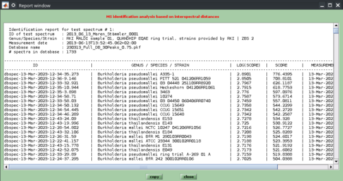
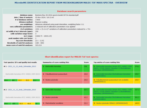
The results of the pattern matching analyses are provided as a score ranking list, either in a text, or a HTML format. In both types of lists, the top matching database entries are displayed on top position. Further records are listed below according to the scores achieved (see screenshots below).

While reports in the simple text format cannot be printed, HTML reports are printable for documentation purposes by using the appropriate function of the webbrowser software (Microsoft Internet Explorer, Mozilla Firefox, Opera, etc.). In cases where a pdf printer driver is available reports can be directly converted into a pdf format. Furthermore, all HTML reports are stored per default in a subfolder /report which is automatically created in the program's root directory (Windows). The name of the HTML report file will be of the format report-cmpr-DAY-MONTH-YEAR-HOUR-MIN-SEC.html, for example report-cmpr-19-Jun-2015-11-36-39.html.

Automated workflow for the comparison of mass spectra against a spectral database

MicrobeMS allows identification of microorganisms based on MALDI-TOF mass spectra and mass spectral libraries by an automated and a manual workflow. This section describes the necessary procedures and steps required for automated identification.

1. Load the mass spectral data files via the load spectra (Bruker data file format), import spectra from mzXML data, or the load MS multifile options of the File menu bar.
2. For identification select the respective spectra in the listbox in the top left corner (the listbox is labeled by MicrobeMS spectra ID`s). To select multiple spectra hold the <shift> key while selecting.
3. Start the automated identification procedure by pressing the button standard ID in the ANALYSIS tab (bottom of the main figure), or by choosing standard ID from the Analysis menu bar. The shortcut for this function is <Shift> + I. MicrobeMS performs then quality tests, automated pre-processing and auto peak picking using the parameters defined in the configuration file of MicrobeMS, microbems.opt. Note that existing pre-processing data and peak tables are not overwritten by this function.
4. When pre-processing / peak detection has been completed MicrobeMS will load the mass spectral database defined in microbems.opt and open a figure labeled as identification analysis based on interspectral distances (see the section Introduction at the top of this page. If the database cannot be loaded (e.g. because of wrong settings in microbems.opt) the programs offers to load this file manually.
5. In the identification window modify the parameters and settings used for distance calculation then press compare (bottom, left). Press this button immediately to start the identification procedure with the default settings. Depending on the number of spectra and the size of the database the computation time may vary between a few seconds and several minutes. A progress indicator will be shown to give an idea of the work remaining. For a description of the parameters and settings see the section above.
6. When classification has been finished the buttons more results, Excel reports, text reports and HTML reports will be activated. Press either of them to see the reports (please refer to the section Visualization and Interpretation of the Results for more details).

Manual workflow for the comparison of mass spectra against a spectral database

In this chapter the manual workflow for identifying microorganisms based on their MALDI-TOF mass spectra and mass spectral libraries is described.

1. Load the mass spectral data files via the load spectra (Bruker data file format), import spectra from mzXML data, or the load MS multifile options of the File menu bar.

2. Manual spectral pre-processing: select first the respective spectra in the listbox in the top left corner (the listbox is labeled by MicrobeMS spectra ID`s). Hold the <shift> key to select multiple spectra while selecting. Spectral pre-processing can be started by pressing the appropriate buttons of the functions smooth (smoothing of spectra), baseline (baseline subtration), normalize (normalization), or calibrate (auto-calibration). Additional pre-processing procedures which can be applied to the spectra before peak picking are cut spectra and reduce resolution. Both functions are available from the Pre-processing menu bar. Recommended spectral pre-processing routines before peak detection are (Bruker spectra in the m/z range 2000 - 20,000):
   a) Smoothing with 21 smoothing points  
   b) Baseline subtration (number of intervals: 60 - 100)
   c) Normalization (no parameters required)
   In selected cases additional pre-processing procedures may be useful.

3. Perform manual peak detection

4. Note that spectra selected for identification should contain valid peak tables. Spectra without associated peak table cannot be processed

5. Start the identification procedure by pressing the button compare with database in the ANALYSIS tab (bottom of the main figure), or by choosing compare with database from the Analysis menu bar. The shortcut for this function is <Shift> + H. MicrobeMS will then open a figure labeled as Identification analysis based on interspectral distances (see the section Introduction at the top of  this page). 

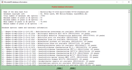
6. Load a mass spectral database by pressing the load button. After loading the content of the database can be printed in the command line window by pressing the button show DB content. Use unload to unload the database.

7. In the identification window modify the parameters and settings used for distance calculation then press compare (bottom, right). Press this button immediately to start the identification procedure with the default settings. Depending on the number of spectra and the size of the database the computation time may vary between a few seconds and several minutes. A progress indicator will be shown to give an idea of the work remaining. For a description of the parameters and settings see the section above.

8. When classification has been finished the buttons text report and HTML report will be activated. Press either of them to see the reports (please refer to the section Visualization and Interpretation of the Results for more details).

Useful links

• Example of a HTML formatted identification report: https://wiki.microbe-ms.com/uploads/report-maldireport-15-Dec-2024-11-06-14.html
• Description of how to modify the default settings for parameters used for auto-preprocessing and auto-peak detection in the microbial identification workflow
• Create database spectra from series of microbial mass spectra
• Description of the format of database spectra
• Description of the format of peak tables
• Description of identification report files (*.xls, *.mat)